Wrapping Up

TL;DR A recap of my work as part of OpenAI’s scholar’s program. I introduce the ‘test time compute dream’ and recap some of the early ways in which I attempted to explore this problem. I detail how attempts to realize the test time compute dream in the form of baking recurrence back into language models were largely unsuccesful. As a means to find signs of life, I transition to graph neural networks operating over the game of sudoku and find definitive signs of life. I also find that using the machinery from deep equilibrium models to refine the hidden state of a graph neural network works quite well for improving training speed and reducing memory footprint. Additionally, I find that instead of explicitly hand-coding the adjacencies for a graph neural network we can instead use an attention head from a transformer to learn the adjacencies from the raw unstructured data and then train this model end to end via a surrogate loss and reinforcement learning.

At long last

Wow, where to begin? The last couple of weeks have been a whirlwind but at long last i’ve arrived at the end of the scholar’s program.

This blog post will largely be a written version of my presentation with about as much detail. To recap, for all two of you who actually read this blog (hi, mom 👋! ),my scholar’s project has been spent thinking about what i’ll call the test time compute dream. Briefly: Can we construct models that continuously improve their outputs the more compute we pout into them at test time?

Recurrence Alone is Inadequate

Broadly I tend to mentally partition test time compute ideas from literature into two general categories..

1. Generalization Improvement mechanisms: These deal with the question of whether we can create models that leverage test time compute to learn more general algorithms instead of simple statistical association. Ideally, we’d like for to construct algorithms that use the extra compute to resolve ambiguity or to refine their outputs using computation they’ve already done or outputs they’ve already produced as new inputs for future time steps. Ideally we would like to have some guarantees that these models are truly computational complete. The Universal Transformer is my canonical example of work in this category.

2. Efficiency Mechanisms: This largely deals with the question of whether we can decouple the amount of time it takes to run a model at inference from the number of parameters a model has. The motivation here is simple; we would like to increase the representational capacity of our model by increasing the total number of trainable parameters without simultaneously incurring increased computational penalty for those extra parameters. Examples of literature of this variety includes eternal memory mechanisms (fast product keys etc)¹

By in large, this project largely focused on the former mechanism.

Particularly, for the first two thirds of this project I was interested in exploring the generalization properties of test time compute methods in the context of the “shortest path dataset” . I’ve talked about the shortest path set several times on this blog, so I wont go into too much detail here. The important question being explored was whether, if we control for total training FLOP budget, does a model trained to leverage test time compute (in the form of top layer recurrence) ever approach the performance of a model that doesn’t use this recurrence but perhaps is larger or was trained for more total gradient steps overall.

The way I did this was by keeping the training budget fixed and then training recurrent models with a fixed number of time steps during training with loss evaluated at every time step and then evaluating those same models with more steps of recurrence at test time. What I was interested in here was whether we ever observe a phase transition whether the extra compute allows these models to catch up with larger models trained without this recurrence.

Obviously theres much nuance here – the very nature this experiment has questionable foundations – regardless, to the extent to which we can answer the question above, the answer seems largely to be: not really. That is, irrespective of the model type you attempt this scheme on (and I tried a wide array of models indeed) we never observe a phase transition where it becomes favorable to expend your training budget on training a model that uses this recurrence scheme over just training a non recurrent model for more gradient update steps.

Running a linear probe over the embedding space of these models reveals that they actually learn the locations of the cities fairly quickly (or at the very least something isometric to the locations). The trouble really does appear as though learning some general shortest path finding algorithm seems to be a sufficiently difficult task for all these state of the art models. Even if you argue that cross entropy loss or perplexity is a poor metric to measure performance on something like shortest path, their performance is actually even worse on more sensible metrics.

To be clear, we really don’t care at all about actually solving the shortest path task, it exists almost solely as a vessel to explore some of these test time compute generalization properties. The actual, absolute, performance on the dataset is largely irrelevant, what matters is the relative performance between models using test time recurrence and those models not leveraging it.

These negative findings hold true to domains outside of shortest path as well. Admittedly, the experiments here were much less extensive but this trend seems to be true even for tasks like sorting (even when models are trained with more than the \(n \log n\) recurrence steps we know are algorithmically sufficient for this domain). It really does appear as though test time compute in the form of recurrence is insufficient to achieve the generalization properties we seek. More structure is required.

Graph Neural Networks to the rescue

In search of this additional structure, I turned to graph neural networks.

.

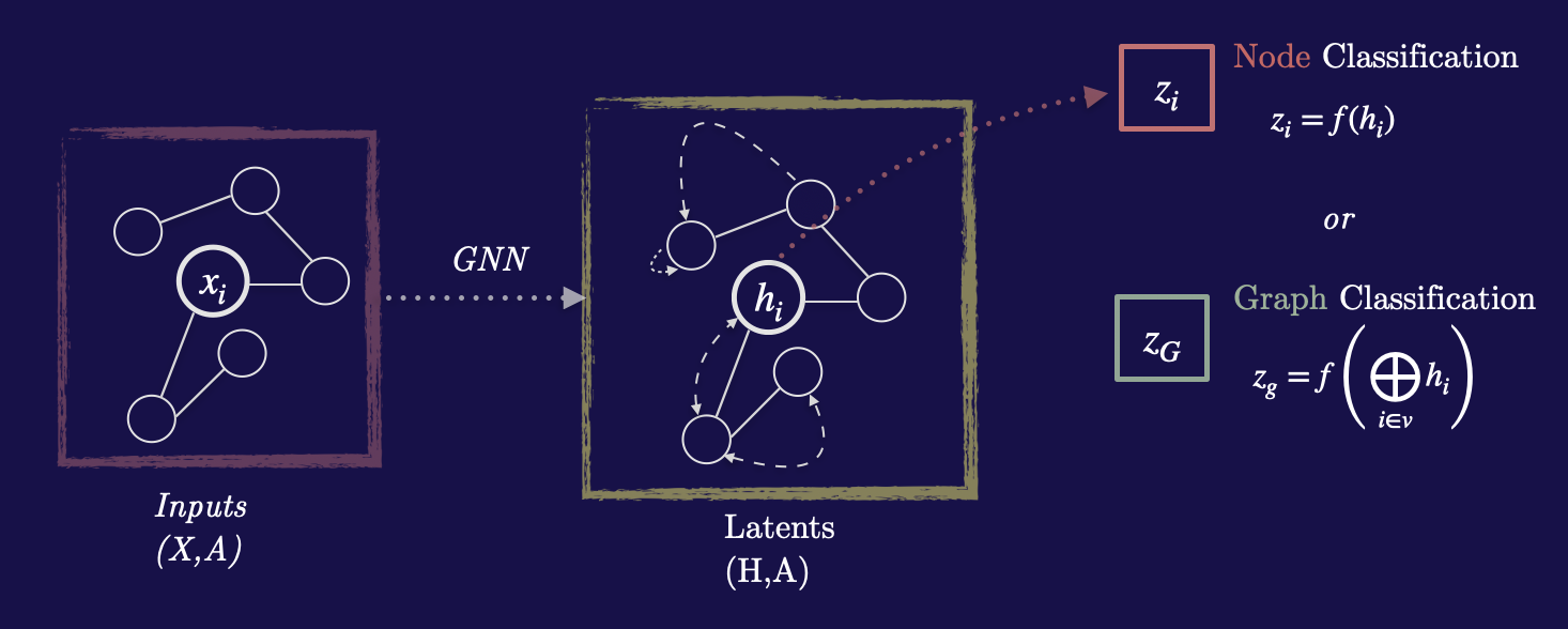
Graph neural networks are neural networks that operate on graph structured data².

GNNs process this graph by iteratively performing a learned message passing operation between nodes in which the GNN attempts to refine it’s internal representation of the nodes. It does this by using a learned message passing mechanism where at each timestep the hidden state is updated in the following way:

Above, \(h_i\) is the hidden state for some node i, and \(x_i\) is the node embedding for a particular node. Effectively, the update equation specifies that the hidden state at each layer (or time step in our case) be updated by a function that takes in as inputs the node embedding, and all pairs of that nodes neighbors passed through some message passing function \(\psi\) and then aggregated using some aggregation function.

The training regime was done in effectively the exact same way as the shortest model explorations where I force the model to make a prediction at every timestep and evaluate the loss at every timestep as well. This is done to ensure that the model is robust to being evaluated at test time with more evaluations than the model was evaluated with during training time.

Signs of Life

.

Above I embedded a movie of this GNN operating over some of the sudoku dataset. What’s particularly interesting is that it seems to prioritize using the extra test time compute (graph refinement steps) to attend to tokens it had previously assigned high uncertainty (low probability) to in the previous time steps. In other words red things become green and green things tend to remain green. This is fascinating because it suggests that the probabilities we extract from the logits seem to have some semantically meaningful concept of uncertainty.

Of further interest is that fact that this GNN actually seems to do better the more iterations you give it. Particularly, if you evaluate it with more iterations than those it was trained with it continues to improve it’s accuracy in an almost monotonic way. Additionally, if you evaluate it on problems that are harder than the problems it was trained on, it actually still does reasonably well (check out the presentation for the actual graphs).

While nothing in the above is particularly novel, it does demonstrate that at least in principle the test time compute dream is possible. The key ingredient here seems to be related to the recurrence plus the message passing mechanism of these graph neural networks.

Can we do better? DEQs to the rescue

If the central argument here is more test time compute in the form of iterations seems to be helpful what if we could take this argument to the infinite limit. In order to do this we need to steal the machinery from deep equilibrium models. I’ve written about deep equilibrium models several times before on this blog³, but the main take away here is that the graph refinement equation for graph neural networks is exactly a fixed point equation which means that the implicit function theorem allows us to use some arbitrary black box root finding algorithm to both evaluate the value of the function at the equilibrium point and the value of the gradients there as well.

Trying this out, works surprisingly well, at first. The deep equilibrium GNN both trains much faster, seems to have better accuracy, and has lower memory requirements than the traditional GNN.

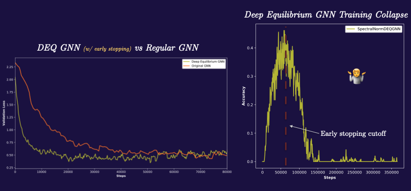
All is not well in paradise however; every single time I’ve trained this model, i’ve observed a strange crash in the training accuracy occur several hours in. The DEQ GNN will train with better accuracy than the traditional GNN, and then all of a sudden die wherein the accuracy plummets to zero. I’m still investigating this and while I have some suspicions about the cause (particularly instability caused by the growth of the spectral norm of the operators) it could also very well be a bug in my training loop. Either way, just mentioning these things here for the sake of completeness.

Learning Graph Adjacencies Using Policy Gradients

All the above is well and good, however, there’s something a little strange about the way I’ve seen graph neural networks used - the fact that the adjacencies must be encoded by hand. For the sudoku problem in particular, I had to explicitly bake in the fact that nodes that share a row, column or a cell are connected. Could we instead learn the adjacencies from the raw unstructured data?

Here’s the idea: transformers are fairly adept at learning how relevant pairs of tokens are to each other. On the other hand GNNs seem to be good at performing well on relational reasoning style tasks particularly over graph structured data. What if we could use the attention head from a standard transformer to extract an adjacency matrix which we then feed into a GNN.

This scheme operates by first feeding our input into a small transformer which has a small modification in the top layer such that we use the probability scores to categorically sample the top K indicies which are most relevant (i.e for each input token what are corresponding k other tokens which the attention head assigns the highest normalized probability to). This then extracts K neighborhoods for each token which we than feed into our GNN.

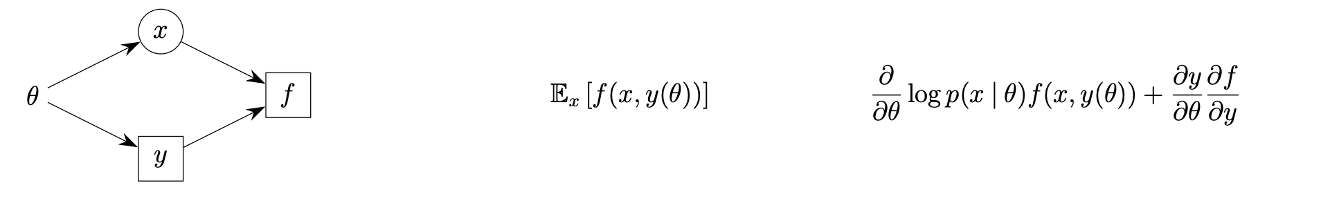
Because sampling indices is a non differentiable operation, we need to compensate for this by using a gradient estimator. John Schulman has a great paper⁴ describing exactly how to do this in the general case for stochastic compute graphs.

.

The formalism outlined in the paper gives us a way to convert stochastic computation graphs into deterministic compute graphs and evaluate a “surrogate loss” that provides a mechanism to use standard backprop to arrive at an unbiased gradient estimator through these stochastic nodes.

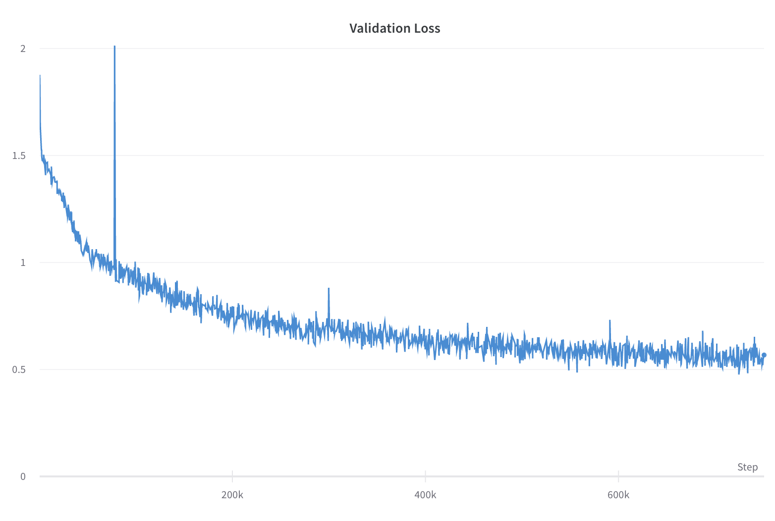
If you try all the above out it kind of works! Works in the sense that the model will achieve low training loss (as well as low validation loss). In reality however, there are several caveats here. The most obvious being the much slower training. Training this Frankenstein stochastic graph transformer took about 5 days compared to the 5 hours of training required for the traditional GNN. Additionally, performance is actually worse that the standard GNN –peaking at 62% best accuracy. Lastly, using vanilla policy gradients in this way has really high variance.

These objections and caveats aside, the interesting thing here is that this demonstrates that in principle one could train a GNN with adjacencies learned from scratch as well. I can imagine this being useful in a number of ways, particularly in contexts where its useful to use the strong relational reasoning performance of graph neural networks but we’d like to learn the graphs dynamically or in a context dependent way.